A Software Solution for Automatic Optimization of Logistics During Well Drilling and Flowback Operations

Optimizing logistics during drilling and the development of wells, consists of building an optimal schedule for all the labour resources. Optimized scheduling makes it possible to significantly reduce the time and costs associated with geological and technological risks. The article describes the functionality of our software solution and presents the results of its testing. The method we used in that project

for optimized scheduling is a combination of well-known algorithms – the branch and bound method and the simplex method. The input dataset is an “Initial Schedule,” which contains the following information: field geometry (the placement of wells and the distance between them); job type list (type of job, its assignment to a particular well, start date, work duration, etc.); schedule admissibility restrictions (job sequencing conditions for one single well, conditions for performing simultaneous work on neighboring wells, etc.). The program allows the user to select the parameter based on which the optimization will be performed, the computation time, and the optimization scenario. At the output, we receive a list of jobs specifying their type, work start date, duration, and assignment to wells. In addition, we receive the total production rate and cumulative production values as at the time of the well pad commissioning in comparison with the original and optimized schedules.

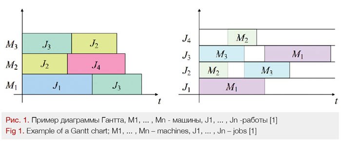
For a convenient graphical representation of the schedule, the program uses Gantt charts [1]. These charts come in two types: equipment workload per job type over time and job types performed on specific equipment. A typical example of a Gantt chart is shown in Figure 1.

An important limitation on optimized scheduling is the need to use a finite time step. This allows us to formulate problems in terms of discrete programming. Here, a discrete programming problem means the problem of minimizing a certain function on a set of feasible solutions.

Our module is based on a variation of the simplex method and the branch and bound method. The branch and bound method is part of a family of pruned-enumeration methods [2, 3, 4]. J. M. van den Akker et al. [4] studied the job prioritization parameters for parallel machine scheduling and evaluated the criteria used for specific tasks. In [3], the authors developed an algorithm for obtaining approximate solutions to the problem of processing time minimization with an increase in accuracy depending on the computation time. Alex J. Ruiz-Torres et al. [2] presented an algorithm for minimizing the processing time on one machine.

The constraint integer programming domain includes several programming areas. Tobias Achterberg et al. [5, 6] provide an overview of constraint integer programming algorithms that are currently of interest. One method that is best-known and most widely used for practical tasks that have to do with solving the general problem of constraint programming is the simplex method. The problem is to optimize a linear functional on a multidimensional space with given linear constraints.

The constraints imposed on variables form a bounded region that is a multidimensional polyhedron. The solution to the problem is one of the vertices of the polyhedron, and the search is iterated through its adjacent faces. Studies conducted in [7, 8, 9] showed a high versatility of the simplex method.

Formulating the Problem

As previously mentioned, to solve the problem, we must select a finite time step. In this formulation, we used a step equal to one day and a total schedule length equal to 365 days to achieve a good trade-off between speed and accuracy.

The field’s multi-well pad comprises 24 wells grouped into clusters of 4 wells each (Fig. 2), the distance between wells in a cluster being 5 meters, and the distance between end-wells of adjacent clusters being 15 meters. The workforce comprises 5 types of crews: drilling – 1 crew, workover – conditionally unlimited, hydraulic fracturing – 1 fleet, coiled tubing – 1 fleet, “Hookup” – 1 crew. What sets the “Hookup” job type apart is that these jobs are carried out simultaneously on the entire cluster. The distance between any two crews should not be less than 30 m, except for jobs of the “Hookup” type, for which the distance is 25 m.

Each crew is assigned its own list of jobs. The total list of jobs consists of 8 operations: (drilling the conductor section, drilling the production section, drilling the liner section) – the drilling crew, (preparing for hydraulic fracturing, flowback) – the WWO crew, (conducting hydraulic fracturing) – the HF fleet, (coiled tubing) – the CT fleet, (“Hookup”) – the “Hookup” crew.

The end goal of optimization is to minimize or maximize the target function. In this paper, three parameters are optimized:

• Maximizing cumulative production: 1) at the end of the year, 2) for the calculated period – 365 days.

• Minimizing the average value of the well commissioning time (RRSU – Rig Release to Startup).

• Minimizing the downtime of critical resources (jobs like “frac” and “coil”). Jobs of this type need to be scheduled as tightly as possible across the entire well pad to reduce their cost.

Software Solution

The solution is designed as a software package. The software package has an interface consisting of 6 main panels shown in Figure 3.

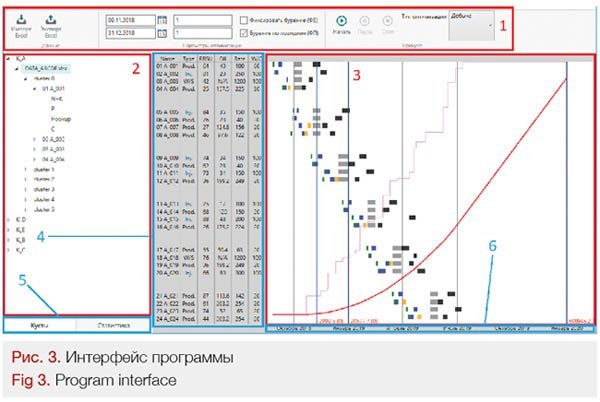
Toolbar (1) features input and output control functions, optimization parameters, and the start function that directly launches the optimization process. Data window (2) allows the user to view schedule data as a tree or as a table of statistics. The display mode is switched using data panel (5). Schedule visualization window (3) displays the data in the form of a schedule broken down by well. The color of the rectangle indicates the type of job, its position indicates the time frame. Besides the jobs, this window shows the production rate figures calculated per day and as a cumulative total. Brief information about the well is available in data table (4). For each well, it contains: its name, type, commissioning time, production rate, and water cut. If necessary, you can set a convenient time base using time scale (6).

Testing

To test the developed software, we used data for 5 well pads (A, B, C, D, E) which were available in the form of an initial schedule broken down by well.

Table 1 shows a comparison based on four optimization parameters: total production until the end of the year (December 31, 2017), total production until the end of the period (365 days from the start of work), downtime days, and average days required to commission a well (RRSU).

In the first optimization variant, the computation time is 10 seconds, in the second one it is increased to 30 seconds.

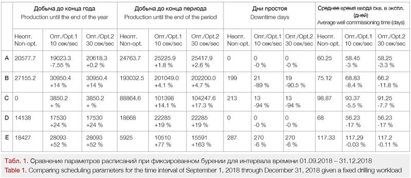
As we can see, in most cases the optimization parameter is improved. However, example A-Opt. 1 for “Production until the end of the year” shows a decrease in the parameter value. This is due to the peculiarities of the optimization algorithm, or, more specifically, its running time. Comparing Opt. 1 and Opt. 2, we can observe that an increase in the computation time improves the optimization performance.

However, there is also considerable scattering of the relative values of the optimization results for different pads, which can be explained by the fact that, in general, the quality of optimization depends not just on the computation time, but also on the complexity of the model and the initial schedule parameters.

Conclusions and Results

The created software package implements its objectives and optimization scenarios given the limitations set forth in the problem formulation statement.

The testing of the optimization model showed improvements in performance relative to the initial schedule by: +163 % in terms of production, -94% in terms of downtime days minimization, and -17% in terms of well commissioning time.

At this stage, the number of tasks for which this model is suitable is quite limited. What needs to be done in this regard is generalizing the problem formulation statement and expanding the model functionality.

Here are some avenues for further expansion of the model:

• Adding functionality for working with input and output data formats;

• Generalizing the model geometry (distance between wells, grouping into pads, into clusters);

• Introducing job-specific risks and costs;

• Introducing preparation jobs and equipment handling jobs;

• Making the time step smaller;

• Accounting for the decline in production over time, accounting for well interference;

• Introducing product prices into the optimization scheme.

Bibliography

1. У. Кларк. Графики Гантта. Учёт и планирование работы. 5-е издание. – Москва: Техника управления. – 1931. [W. Clark. Gantt charts. Work accounting and planning. 5th edition. – Moscow: Tekhnika upravleniya. – 1931.]

2. Alex J. Ruiz-Torres, Giuseppe Paletta, Eduardo Pérez. Parallel machine scheduling to minimize the makespan with sequence dependent deteriorating effects. Computers & Operations Research 40 (2013) 2051–2061.

3. Klaus Jansena, Monaldo Mastrolilli. Approximation schemes for parallel machine scheduling problems with controllable processing times. Computers & Operations Research 31 (2004) 1565–1581

4. Van den Akker J.M., Hoogeveen J.A., van de Velde S.L. Parallel machine scheduling by column generation // Oper. Res. – 1999. – V. 47, N 6. – P. 862–872.

5. SCIP: Solving Constraint Integer Programs Tobias Achterberg. Mathematical Programming Computation, Volume 1, Number 1, Pages 1–41, 2009.

6. Constraint Integer Programming: A New Approach to Integrate CP and MIP. Tobias Achterberg, Timo Berthold, Thorsten Koch, Kati Wolter, Integration of AI and OR Techniques in Constraint Programming for Combinatorial Optimization Problems, CPAIOR 2008, LNCS 5015, Pages 6–20, 2008

7. Bland, Robert G. (May 1977). “New finite pivoting rules for the simplex method.” Mathematics of Operations Research. 2 (2): 103–107

8. Maros, István (2003). Computational techniques of the simplex method. International Series in Operations Research & Management Science. 61. Boston, MA: Kluwer Academic Publishers. pp. 325

9. Spielman, Daniel; Teng, Shang-Hua (2001). “Smoothed analysis of algorithms: why the simplex algorithm usually takes polynomial time.” Proceedings of the Thirty-Third Annual ACM Symposium on Theory of Computing. ACM. pp. 296–305.

Authors:

D. M. Khamadaliyev,¹ Ye. N. Ulyanov,¹ V. N. Ulyanov,² D. O. Taylakov,² K. S. Serdyuk,² R. Z. Kurmangaliyev,² S. A. Frolov,² K. I. Nektyagayev,² R. I. Vylegzhanin,² Ye. N. Pavlovsky³

1. Salym Petroleum Development N. V.,
2. Novosibirsk Scientific and Technical Center, LLC,
3. NSU Laboratory of Data Streaming Analytics and Machine Learning