
Fundamentals of Subsurface Hydrodynamics and a Quantum-Mechanical View of the Reservoir Model
1. Tim’s Theorem. The fundamental dependences of the key hydrodynamic parameters of the reservoir and the well and their interrelationships as the basis for a new paradigm of subsurface hydrodynamics
The “Producing Reservoir – Well – Pumping (Lift) Equipment” system is a uniform, inseparable hydrodynamic system interconnected by fundamental dependences reflecting on the uniformity and interconnectedness of all the hydrodynamic parameters of this system [4]. The near-wellbore region of the reservoir is a special zone characterized by high activity and unstable energy dynamics. Such processes as drilling the first well into the pay zone, well completion, and subsequent well operations upset both the mechanical energy equilibriums and the electrodynamic equilibrium in the formation. Both the hydro-thermodynamic and physico-mechanical characteristics of the near-wellbore rock change, as do the reservoir fluid properties in this region. Physico-chemical and chemico-biological transformations take place. The reservoir’s electrodynamic equilibrium is upset, and, because of this, hydrogen bonds, acting as retention mechanisms for the hydrocarbon systems, begin to form in the capillaries and fractures of the near-wellbore region, and the bond energy, as determined by the van der Waals forces and electrical double-layer (EDL) interaction force fields, are redistributed. All these production-related processes and other factors, the list of which above is nowhere near complete, significantly affect the physico-rheological parameters of the reservoir fluid and impair the permeability and porosity of the near-wellbore area, forming a layer with non-uniform permeability and porosity distribution called the skin zone and produces a several-fold reduction in the rate of fluid flow into the wellbore.
A. F. van Everdingen and N. Hurst (1949) proposed formula (1) for calculating the pressure drop occurring in the near-wellbore area as the fluid flows into the wellbore [1].
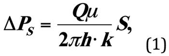
where ΔРs is the incremental reservoir pressure drop that occurs during the filtration of fluid into the bottom-hole region due to the impairment of reservoir permeability in the skin layer from k to ks; µ is the dynamic viscosity of the reservoir fluid Q; S is the skin factor value. The parameter ΔРs is important and is included in the derivation of the formulas for all the key hydrodynamic parameters of a multi-zone heterogenous reservoir.
It should be noted that an analytical derivation of expression (1) does not exist, and on top of that, the following gross errors have been made:
• firstly, according to the laws of oil reservoir hydrodynamics governing the process of fluid filtration, the value of ΔРs has a logarithmic nature, i. e. ΔРs changes along a logarithmic curve, and formula (1) fails to take this into account. This serious error introduced uncertainty and ± ∞ into the S value;
• secondly, the pressure drop ΔРs depends on the value of the skin layer radius (thickness) Rs, and formula (1) fails to take the skin layer thickness Rs into account. This contradicts the laws of reservoir hydrodynamics and significantly distorts the actual value of S;
• thirdly, the skin layer permeability factor ks is not accounted for in the determination of ΔРs, since ΔРs is the incremental filtration-related pressure loss in the skin zone with permeability factor ks, which means that the value of the coefficient ks should be considered. This gross error led to a complete distortion of the value of S.
Thus, formula (1) proposed by A. F. van Everdingen and N. Hurst (1949) for determining ΔРs fails to observe the physical laws governing the reservoir hydrodynamics, violates mathematical logic, and contains the serious errors set forth above. M. F. Hawkins (1956), using (1), proposed the following formula for calculating S: (2), which has been introduced into educational and scientific literature as Hawkins’ formula [2].
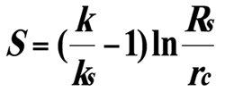
According to this formula, S can take values from minus infinity to zero and from zero to plus infinity, i. e.
![]()
without belonging to a particular domain of definition, existence, or practical use. It is known that if a function tends to infinity, it has no practical application.
Subsurface hydrodynamics as an independent branch of petroleum science, founded and organized by Russian scientists N. Ye. Zhukovsky, N. N. Pavlovsky, L. S. Leybenzon, S. A. Khristianovich, V. N. Shchelkachev, et al., as well as by foreign scientists M. Muskat, Van A. F. van Everdingen, N. Hurst, and M. F. Hawkins, seemed to have taken its final shape by 1950s with even the last finishing touches having been put to the fundamental whole of this science. Here, “final” means that the key laws of reservoir fluid filtration hydrodynamics that govern the subsurface processes occurring in an oil and gas formation have been discovered, relevant equations and solutions to them have been written. There was no reason to doubt the reliability of the principles of this science that we all knew. Any branch of science that is rapidly developing should do more than just formulate and establish the basic principles on which it is built: the main focus areas and limits of applicability of these principles should also be established.
No matter what theoretical and technological successes modern science may have attained in terms of reservoir hydrodynamics, it is far from perfect and, by the end of the 1950’s, it had almost completely exhausted its potential. Since that time, no fundamental theories have been created, and the conceptual developments that took shape along the main avenues of application have indeed gone the wrong way.
What comes as a bitter surprise is the fact that, for more than five decades at the beginning in the second half of the 20th century, the patriarchs of Russian and foreign petroleum sciences were convinced of the infallibility of the formula in (Van Everdingen & Hurst, 1949) for determining ΔРs, the formula in (Hawkins, 1956) for determining the skin factor S, as well as the formula used for determining the influx rate Qs to the bottom-hole region of a real-world well, despite the obvious errors in, and controversies around, these formulas, which were all made up with gross violations of the laws of subsurface hydrodynamics.
The negative consequences of these errors and delusions have been reflected in the theory and practice of the fundamentals of hydrodynamic well testing (GDIS), geophysical well logging (GIS), and mud logging (TIS), but something we can really describe as a disastrous effect is the fact that, since the second half of the last century, these formulas have been included in all textbooks, teaching aids, and study guides of universities, colleges, and postgraduate training courses specializing in the subject-matter without any derivations or proofs whatsoever.
Modern subsurface hydrodynamics is ailing from the inside out. The main causes of that ailment, as well as its tenacity and persistence, are a profound stagnation in scientific ideas combined with a dogmatic approach to formulating and solving fundamental scientific problems aggravated by the conservatism of scientific thought. Whatever research work was conducted in the field of subsurface hydrodynamics since that time up until the present day can be reduced to the development of semi-empirical theories whose sole purpose was to tweak the mathematical apparatus to reality and which, as all erroneous concepts, had but preparatory value if any. One example of this is the fact that, to this day, the most fundamental questions have remained open and debatable: what is the domain in which skin factor values S exist, and to which it belongs, and what to do with the uncertainty about the positive and negative signs of its values? Another such issue is the lack of a rigorous theory behind the derivation of its formula. Because of this, numerous issues with the quality of drilling and completion work performed on a reservoir, predicting its energy state and filtration properties, determining its productivity, current and potential flow rates, and assessing the oil recovery factor of the reservoir as a whole have not been resolved. It was a time of deep crisis in the field of subsurface hydrodynamics.
The errors in (1) and (2), as well as errors in the formulas used for calculating the key hydrodynamic parameters of the reservoir, and the discrepancies between the calculations made using the said formulas and the data obtained from field practice and experiments served as an impetus to create a new paradigm for subsurface hydrodynamics – a realistic hydrodynamic reservoir model [3, 4, 7].
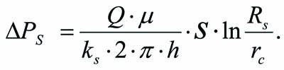
[3, 4] contain a detailed derivation of the following formula for determining ΔРs, taking into account the multi-zone heterogeneity of the reservoir:
There are also indicated are historical errors and misconceptions incorporated into the conventional formulas for determining the skin factor, pressure drop, and influx rate in the skin layer during fluid filtration. In this connection, a detailed and consistent analytical derivation of its formula is given. 1 – The analytical derivation of the skin factor formula is confirmed using five alternative methods, viz deriving through: 2 – “flow rate – pressure” and 3 – “flow rate – level” indicator lines, 4 – bottom-hole pressure and 5 – potential flow rate values; 6 – a formula for the skin factor for a multi-zone heterogenous reservoir is given [3, 4, 5]. A dependence for estimating the influence of the skin layer radius and the permeability factor on the amount of fluid flowing into the wellbore is derived.
The key parameters based on which a hydrodynamic reservoir model can be constructed are the actual value of the pressure drop ΔРs that occurs during the wellbore fluid filtration in the near-wellbore region, the value of the skin factor S, the productivity factor К and the permeability factor k; the reservoir pressure Рпл and the bottom-hole pressure Рз, the dynamic borehole fluid level hд, the current influx rate Qж, the potential flow rate Qпот, and the mathematical formulas for their determination.
Based on theoretical and applied research performed in the field of subsurface hydrodynamics and co-functioning of the reservoir, well, and lift equipment, fundamental dependences have been established and determined for all key hydrodynamic parameters of the reservoir, well, and pumping (lifting) equipment that are required for assessing the state of the near-wellbore region of a reservoir pay zone and for assessing the state of a multi-zone heterogenous reservoir [3…9]
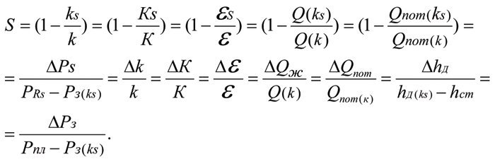
The fundamental dependences (Tim’s formula) for assessing the state of the near-wellbore region of a producing reservoir [4…7] are as follows:
The fundamental dependences (Tim’s formula) for assessing the state of a multi-zone heterogenous reservoir are as follows:
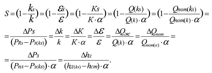
where α is the reservoir heterogeneity coefficient, which is, in fact, a proportionality factor that accounts for how non-homogeneously permeability is distributed within the reservoir.
The words “The ‘Reservoir – Well – Pumping Equipment’ system as a uniform, inseparable hydrodynamic system interconnected by fundamental dependences reflecting the uniformity and interconnectedness of all hydrodynamic parameters of this system” are confirmed by mathematical proofs and derivations for all key hydrodynamic parameters of the reservoir and for their interrelationships via fundamental dependences [3…9]. The latter papers provide detailed and consistent evidence for all the provisions of Tim’s Theorem. Tim’s Theorem states that “Any changes in the reservoir permeability lead to proportional changes in its productivity, hydraulic conductivity, bottom-hole pressure, dynamic fluid level, current influx rate, and potential flow rate, and their dimensionless relative values are equal to each other.”

Fig. 1. A complete geometric interpretation of the fundamental dependences and the interrelationship between the hydrodynamic parameters of the reservoir and the wellbore, confirming Tim’s Theorem, is shown above; 1 is the indicator line Рз=f(Qж(к)); 2 is the indicator line Рз=f(Qж(кs)); 3 is the indicator line hд=f(Qж(к)); 4 is the indicator line hд=f(Qж(кs)); К is the productivity factor at the native permeability of the reservoir, k; Кs is the productivity factor at the impaired permeability of the reservoir, ks; Qж(кs) is the fluid influx rate at reservoir productivity k; Кs is the decrease in productivity resulting from the impairment of reservoir permeability from К to Ks; Qж(кs) is the fluid influx rate at formation productivity Ks; Qж is the decrease in influx rate resulting from the impairment of reservoir productivity from К to Кs; hст is the static fluid level in the wellbore; hд(к) is the dynamic fluid level in the wellbore at reservoir productivity К; hд(кs) is the dynamic fluid level in the wellbore at reservoir productivity Кs; Δhд is the decrease in dynamic fluid level in the wellbore resulting from the impairment of reservoir productivity from К to Кs; L is the well depth up to its top perforations; Lд(к) is the dynamic depth at reservoir productivity К; Lд(кs) is the dynamic depth at reservoir productivity Кs; ΔРз is the decrease in bottom-hole pressure resulting from the impairment of reservoir productivity from К to Кs; Qпот(к) is the potential flow rate at reservoir productivity К; Qпот(кs) is the potential flow rate at reservoir productivity Кs; ΔQпот is the decrease in potential flow rate resulting from the impairment of reservoir productivity from К to Кs.
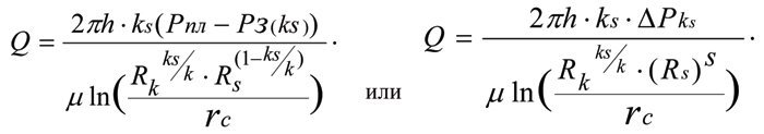
[4–9] provide a critical analysis of the generally accepted formula used for determining the rate of fluid influx to the bottom-hole region of a real-world well, clearly specifying the errors it contains and presenting four alternative derivations of the following formula to be used for determining the rate of fluid influx to the bottom-hole region of a real-world well:
The fundamental dependences (Tim’s formulas) completely describe a realistic hydrodynamic model of a reservoir, and Tim’s Theorem proves its validity.
The fundamental dependences between the hydrodynamic parameters of the “Reservoir – Well – Pumping equipment” system should be used to quantify and fully analyze the state of the reservoir, as well as for purposes of hydrodynamic well testing (GDIS), geophysical well logging (GIS), mud logging (TIS), and comprehensive technological and hydrodynamic feasibility assessments for software development projects to support innovative process design solutions for oil and gas field development.
2. Quantized fields of the producing reservoir as a physical (natural) object in a real, material world
When studying most engineering systems and technological processes, must simultaneously consider the joint effect of mechanical, thermal, electric, magnetic, optical, and gravitational fields, as well as any interrelationships among them. An important factor for establishing the relationships between various physical fields is their conventional dimension taken under a uniform system of units of measurement.
A producing reservoir is exposed to a multitude of changing geophysical fields (multi-fields): geomechanical, hydrodynamic, geomagnetic, electrodynamic, geothermodynamic, gravitational, undulatory, optical, as well as their derivatives. The values of the parameters of these geophysical fields are completely interrelated and depend on the spatial heterogeneity and temporal variability of the state of the entire system.
These fields can be divided into two groups:
1. Geomechanical and hydrodynamic fields. In this case, the term “fields” should be understood to refer to a portion of reservoir rock, which occupies
a certain volume in space and is exposed to lithostatic pressure acting on all sides of it and characterizing its stress state, strength, elasticity, stability, permeability, porosity, reservoir pressure, rheological parameters of the reservoir fluid, etc. For geomechanical and hydrodynamic problems, the concept of a field is used purely as a convention for the purpose of constructing a mathematical model of the working system.
2. Electromagnetic and gravitational fields. These fields, unlike the former group of fields, represent real material objects, viz. elementary particles. The electromagnetic field is governed by elementary particles – electrons, protons, neutrons, quarks – and their decay. There are three fundamental interactions that describe how these particles influence each other. An example of electromagnetic interaction is an electron’s attraction to the nucleus. An example of strong interaction is the mutual attraction of quarks (intra-nuclear interaction). An example of weak interaction is the decay of a quark and a free neutron (beta-decay). In addition to the three fundamental interactions described above, there exists the fourth fundamental interaction playing a huge role in nature: it is the mutual attraction of all particles to each other in a gravitational field. Responsible for this field are elementary particles called gravitons.
Let us call these fields the “quantized fields of the reservoir”. A quantized field is a natural reality, a material object that possesses energy, inertia, and gravity. The totality of lines of force of quantized fields at a given point in space forms the so-called potential field. For a potential field, two important properties hold. The first one is the principle of superposition, according to which the net effect of the group of sources generating the potential field can be found by successively summing up the vector values characterizing the field generated by each source taken separately.
The second important property that holds for a potential field is the maximum principle. The potential function can only reach its maximum or minimum value on the surface of the field source or at infinity.
Quantum electrodynamics (QED) is the quantum theory of electromagnetic interactions, the best-elaborated part of quantum field theory. Classical electrodynamics only considers the continuous properties of electromagnetic fields. Quantum electrodynamics is based on the fact that an electromagnetic field also possesses discontinuous (discrete) properties, whose carriers are the field quanta named photons. The interactions of electromagnetic radiation with charged particles are viewed in quantum electrodynamics as instances of absorption and emission of photons by the particles. Quantum electrodynamics as a fundamental quantum field theory was created in the 1940s in the works of R. Feynman [10]. This was the first interaction field theory describing the behavior of charged elementary particles in a magnetic field. Quantum electrodynamics provides a quantitative explanation for the effects of field-to-matter interactions as well as a consistent description of electromagnetic interactions between charged particles. The electromagnetic field (and its change over time) is described in electrodynamics using a system of four legendary vector equations known as Maxwell’s, where the electric and magnetic fields are regarded as manifestations of just one field referred to as electromagnetic. In quantum mechanics, the total energy of interaction between electrically charged particles is determined by the Hamiltonian operator: for example, the Hamiltonian of an atom with nuclear charge Z has the following form [11]:
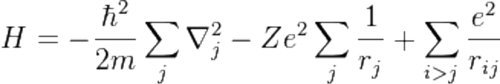
Here, m is the mass of the electron, е is its charge, rj is the absolute value of the radius vector of jth electron, ħ is Planck’s constant. The first term represents the kinetic energy of the electrons, the second term represents the potential energy of the Coulomb interaction between the electrons and the nucleus, and the third term represents Coulomb’s potential energy due to the mutual repulsion between the electrons. The summation in the first and second term is over all Z electrons. In the third term, the summation runs over all pairs of electrons, with each pair occurring only once [12]. Planck’s constant ħ, whose value is fixed and equal to 6.626 x 10⁻³⁴ J·s, is the portion of electromagnetic energy corresponding to one quantum. Planck’s constant ħ defines the boundary between the macrocosm, where the laws of Newton’s mechanics apply, and the microcosm, where the laws of quantum mechanics apply.
Planck’s constant ħ indicates the lower limit of spatial quantities, below which the effects of quantum mechanics should be taken into account.
2.1. Quantum electrodynamics of the reservoir as the basic framework for calculating the structured oil reserves.
The present study is the first-ever attempt to make use of the information value of the electrical double layer (EDL) that forms in the capillaries and fractures of the reservoir rock. The electrical double layer occurs when two phases, one of which is liquid, come into contact. The system’s tendency toward lower surface energy causes the particles at the interface to orient themselves in a particular way. As a result, the contacting phases acquire charges of opposite sign but equal magnitude, which causes an electrical double layer to form (Fig. 2).
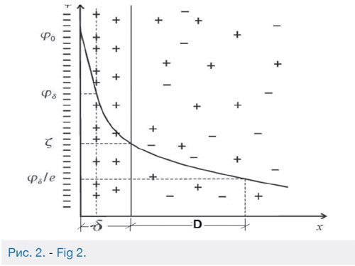
The resulting double layer can be divided into the compact portion δ (Helmholtz layer) formed by ions directly adjoining the surface of the rock capillary wall and the diffuse portion (Gouy layer) D. As a result of electrostatic attraction between the ions and the charged surface, on the one hand, and the chaotic thermal movement of molecules prompting the ions to evenly distribute in the oil, on the other, the ionic portion of the solution acquires a diffuse structure. The concentration of ions carrying a charge opposite to that of the rock surface decreases with distance from the surface, and the concentration of ions having a charge of the same sign as the rock charge increases with distance from the surface (Fig. 2). The Helmholtz layer, also known as the adsorption layer, directly adjoining the interfacial surface has thickness δ equal to the radius of the potential-determining ions [13].
The total thickness of the diffuse layer D depends on a number of fundamental constants:
![]()
where ε is the absolute dielectric constant of the fluid, R is Boltzmann’s constant, Т is the absolute temperature, е is the electron charge, NA is Avogadro’s number, Ci is the concentration of cations of different nature, Zi is the valence of the cations. In this formula, Boltzmann’s constant R is extremely important.
If Planck’s constant ħ defines the boundary between the macrocosm, where the laws of Newton’s mechanics apply, and the microcosm, where the laws of quantum mechanics apply, the constant R establishes a direct relationship between the characteristics of the microcosm and the characteristics of the macrocosm. In charge of this relationship is Boltzmann’s constant R, which is equal to 1.38 x 10⁻²³ J/K. The total thickness D of the diffuse layer is difficult to determine. The value that is used for practical calculations is the so-called effective thickness λ of the diffuse portion of the EDL. The effective thickness of the diffuse layer, λ, is the distance at which the potential existing at the boundary between the compact and the diffuse layers drops е (the base of natural logarithms) times.The diffuse layer, or the Gouy layer, in which the counterions are located, has thickness λ, which depends on the properties of the system and can become quite large. The value of λ is determined for purposes of mathematical description of the EDL using the following expression:
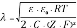 (4)
(4)
where ε is the dielectric constant; R is the gas constant, 8.3 J/(mol·K); Т is the absolute temperature; Z is the ion charge; F is the Faraday constant, 96400 C/mol; С is the concentration of ions, mol-ion/l; ε0 is the electric constant, 8.85 x 10⁻¹² F/m.
The thickness of the compact layer δ (the Helmholtz layer) is determined based on the value of the potential-determining ions. The effective thickness of the diffuse layer, λ, is determined using formula (4). The total thickness of the EDL ranges between 1.5 and 8.5 μm [13]. The average values of δ and λ are used to construct a capillary oil-flow velocity profile covering the entire influx rate value range (Fig. 3 & 4). The preliminary values of oil content have been determined based on structural parameters.
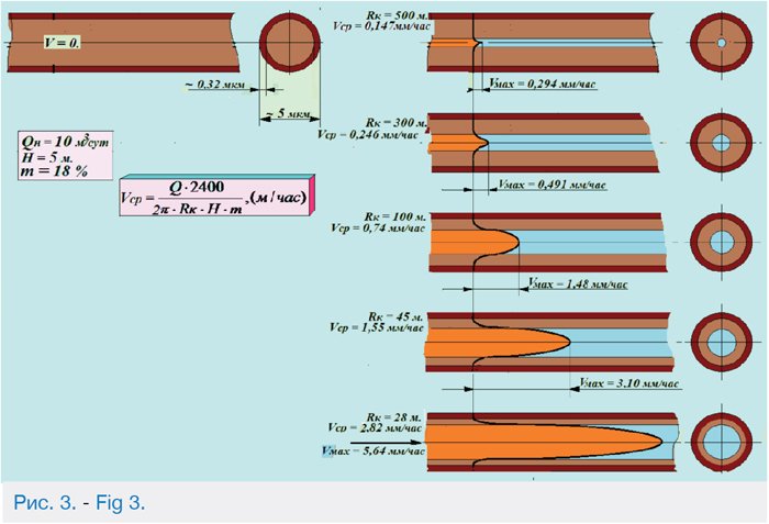
Fig. 3 Changes in the flow profile and thickness profile of the diffuse layer at different capillary oil-flow velocities for a capillary diameter of 5 μm.
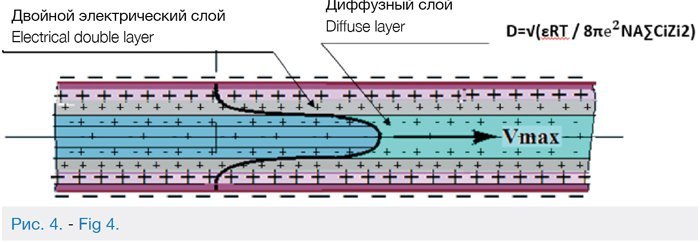
Fig. 4 shows a schematic diagram of an electrical double layer in the capillaries of the rock, comprising a Helmholtz layer and a diffuse layer.
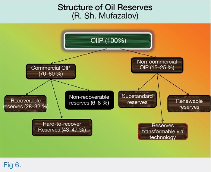
The Helmholtz layer δ is the immobile (solid) wall-boundary layer containing oil that absolutely cannot be extracted. In terms of volume, this layer accounts for 6–8 % of Oil Initially in Place (OIIP) and is fully included in Commercial Oil in Place (COIP) volumes.

The high-viscosity, low-mobility intermediate oil layer that forms the transition boundary between the Helmholtz layer and the diffuse layer D comprises some 20–25 % of OIIP. This volume can be classified as a practically non-recoverable portion of oil reserves given the current state of development of production equipment and technology. Moreover, this layer is still strongly influenced by the attraction of charged particles from the compact double Helmholtz layer.
The transition layer, which should be classified as hard-to-recover, is located at the ‘take-off’ region of the diffuse layer D, starting from which the forces of mutual attraction between charged particles begin to decrease exponentially. The size of the hard-to-recover portion is 25–32 % of OIIP.
The mobile layer of oil constitutes the readily recoverable portion. Here, the concentration of ions carrying a charge opposite to that of the rock surface decreases with distance from the capillary wall, and the concentration of ions having a charge of the same sign as the rock charge increases. The forces of attraction and repulsion generated by charged ions are neutralized.
The size of the mobile, readily recoverable portion is 25–32 % of OIIP, or 35–45 % excluding the Helmholtz layer.
The oil reserves structure shown below (Fig. 6) combines the oil volumes pertaining to the highly viscous low-mobility layer and the transition layer; the values given are percentages of COIP.
Brief information about the author:
Robert Mufazalov
• 270 academic papers, of which:
• 117 inventions;
• 13 monographs (scientific books);
• 4 university textbooks (endorsed by the Ministry of Higher Education);
• Honored Inventor of the Republic of Bashkortostan;
• Inventor of the USSR;
• Excellence Award from the Ministry of Oil Industry of the USSR;
• Included in the encyclopedia «Ural Engineers»;
• Corresponding Member of the Academy of Natural Sciences;
• Participant of more than 30 international conferences, congresses, and international exhibitions on the latest and research-intensive technology.
Academic interests:
Quantum geomechanics, subsurface hydrodynamics, hydraulics, nonlinear hydroacoustics, drilling equipment and technology, oil production hydromechanics, petrochemistry, development and creation of high technology for the petrochemical complex.
Bibliography
1. A. F. van Everdingen and W. Hurst. The Application of the Laplace Transformation to Flow Problems in Reservoirs. – Trans. AIME, Vol. 186, 1949. – pp. 305–24.
2. M. F. Hawkins, Jr. A note on the skin effect. – Trans. AIME, Vol. 207, 1956. – pp. 356–57.
3. Муфазалов Р. Ш. Исторические ошибки и заблуждения, допущенные в теории гидродинамики нефтяного пласта и их последствия. Часть 1, 2, 3. // Труды 12 – Международного симпозиума «Энергоресурсоэффективность и энергосбережение». – Казань: «Центр Оперативной Печати». – 2011. – С. 409–464. [R. Sh. Mufazalov. Historical errors and misconceptions at work in the oil reservoir hydrodynamics theory, and their consequences. Part 1, 2, 3. // Proceedings # 12 of the International Symposium titled “Power resource efficiency and power savings.” – Kazan: Tsentr Operativnoy Pechati. – 2011. – pp. 409–464.]
4. Муфазалов Р. Ш. Скин-фактор. Исторические ошибки и заблуждения, допущенные в теории гидродинамики нефтяного пласта. – Георесурсы. № 5. – 2013. – С. 34–48. [R. Sh. Mufazalov. Skin factor. Historical errors and misconceptions at work in the oil reservoir hydrodynamics theory. – Georesources. Issue # 5. – 2013. – pp. 34–48.]
5. R. Sh. Mufazalov. Skin factor and its importance for evaluating borehole environmental conditions for a productive formation. // «ROGTEC», Oil & Gas Magazine. Issue # 19. – pp. 18–36.
6. Муфазалов Р. Ш. Скин-фактор. Фундаментальные зависимости параметров пласта, скважины, оборудования и фундаментальное заключение. // Материалы научно-практической конференции «Актуальные вопросы разработки нефтяных месторождений на поздних стадиях». Уфа: Изд-во УГНТУ. – 2010. – с. 80–93. [R. S. Mufazalov. Skin factor. Fundamental relationships between the reservoir, well, and equipment parameters and a fundamental conclusion. // Materials of the International Research & Practice Conference titled “Topical issues of mature oil and gas fields development.” Ufa: UGNTU Publishing House. – 2010. – pp. 80–93.]
7. Муфазалов Р. Ш. Исторические ошибки и заблуждения, допущенные в теории подземной гидродинамики, и ее новая парадигма. // Материалы международной научно-практической конференции «Инновации в разведке и разработке нефтяных и газовых месторождений». – Казань: Изд-во НПО «Ихлас». – 2016. Т. 2. – с. 58–63. [R. Sh. Mufazalov. Historical errors and misconceptions at work in the theory of subsurface hydrodynamics and a new paradigm for it. // Materials of the International Research & Practice Conference titled “Innovation in the exploration and development of oil and gas fields.” – Kazan. Ikhlas Publishing House. – 2016. Vol. 2. – pp. 58–63]
8. R. Sh. Mufazalov. Skin factor. Relationships, conclusions, and the formula for the key hydrodynamic parameters. // ROGTEC, Oil & Gas Magazine. Issue # 41. – pp. 74–88.
9. Муфазалов Р. Ш. Теорема Тима. Фундаментальные зависимости гидродинамических параметров пласта и скважины, и их взаимосвязь – основа инновационного проектирования процессов разработки нефтегазовых месторождений. // Материалы Международной научно-практической конференции «Моделирование геологического строения и процессов разработки – основа успешного освоения нефтегазовых месторождений». – Казань: Изд-во «Слово». – 2018. – с. 67–69. [R. Sh. Mufazalov. Tim’s Theorem. Fundamental dependences among the hydrodnamic parameters of the reservoir and the well and their interrlationships as a basis for innovative process design solutions for oil and gas field development. // Materials of the International Research & Practice Conference titled “Modeling the geological structure and development processes as a basis for successful exploitation of oil and gas fields. – Kazan. Slovo Publishing House. – 2018. – pp. 67–69.]
10. Фейнман Р. Квантовая электродинамика. 3-е изд. – М.: Наука. – 2004. – 255 с. [R. Feynman. Quantum electrodynamics. 3rd ed. – Moscow: Nauka. – 2004. – 255 pp.]
11. Грибов В. Н. Квантовая электродинамика. – Ижевск: РХД. – 2001. – 288 с. [V. N. Gribov. Quantum electrodynamics. – Izhevsk: RKhD. – 2001. – 288 pp.]
12. Берестецкий В. Б., Лифшиц Е. М., Питаевский Л. П. Квантовая электродинамика. – М.: Физматлит. – 2002. – 720 с. [V. B. Berestetsky, Ye. M. Lifshits, L. P. Pitayevskiy. Quantum electrodynamics. – Moscow: Fizmatlit. – 2002. – 720 pp.]
13. Дамаскин Б. Б., Петрий О. А. Введение в электрохимическую кинетику. 2-е изд. – М.: Наука. – 1983. [B. B. Damaskin, O. A. Petriy. Introduction to electrochemical kinetics. 2nd ed. – Moscow: Nauka. – 1983.]
14. Муфазалов Р. Ш. Квантовая электродинамика пласта – фундаментальная основа подсчета структурных запасов нефти. // Материалы Международной научно-практической конференции «Моделирование геологического строения и процессов разработки – основа успешного освоения нефтегазовых месторождений». – Казань: Изд-во «Слово». – 2018. – с. 296–300. [R. Sh. Mufazalov. Quantum electrodynamics of the reservoir as a basis for successful exploitation of oil and gas fields. // Materials of the International Research & Practice Conference titled “Modeling the geological structure and development processes as a basis for successful exploitation of oil and gas fields. – Kazan. Slovo Publishing House. – 2018. – pp. 296–300.]