Tim’s Theorem: A New Paradigm for Underground Hydrodynamics Part 2
There are thousands of paths that lead to delusion, but there is only one leading to the truth.
Jean-Jacques Rousseau, 1712–1778.
This article is part 2, following part 1 that appeared in ROGTEC Issue 57
This paper presents a critical analysis of the existing concept used to determine the rate of fluid influx to the bottom-hole area of a real-world well in a reservoir characterized by multi-zone heterogeneity and clearly specifies the errors it contains. It outlines four alternative derivations of the formula for determining the rate of fluid influx to the bottom-hole area in a multi-zone heterogenous reservoir. This formula for determining the influx rate is verified by the alternative derivation paths that produce the said influx formula using the bottom-hole pressure values (and accounting for the pressure loss in the skin layer and the external boundary) and the value of the permeability factor in a multi-zone heterogenous reservoir. The paper also specifies the errors made in the formula for determining the effective (equivalent) wellbore radius. It presents a new definition of the effective (equivalent) wellbore radius and provides a derivation of its formula.
3. Errors and misconceptions occurring in the formulas for determining the influx to the bottom-hole region of a real-world well and its equivalent (effective) radius
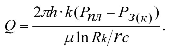
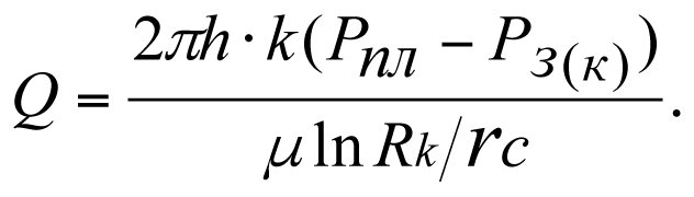
The influx of reservoir fluid to the bottom-hole region of an ideal well with radial two-dimensional filtration flow is determined using the Dupuy formula
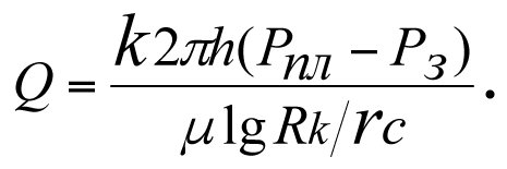 . (3.1)
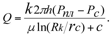
[1, 3,] and other education and scientific publications, including non-Russian ones, recommend that the influx to the bottom-hole region of a hydrodynamically imperfect (real-world) well be determined as
 (3.2)
(3.2)
where S is the value of the skin factor.
V. I. Shchurov [6] recommends (3.2 *) as the formula for determining the influx rate, this formula being no different from (3.2), where the value of C reflects the hydrodynamic imperfection in terms of the degree and character of penetration into the reservoir.
 (3.2 *)
A. I. Ipatov and M. I. Kremenetsky. [4] recommend (9.5.2.2), where
 (3.3)
(3.3)
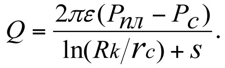
S. N. Zakirov, I. M. Indrupsky, E. S. Zakirov, et al. [5] consider the following formula to be the most rigorous method for determining the influx rate:
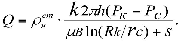 (3.3 *)
Comparing the trivial formulas (3.2), (3.2 *), (3.3), and (3.3 *) with the Dupuy formula makes it clear that the only difference is the additional term in the denominator, S or С. In (3.3), the main determining parameter k is hidden under the ε sign, and in (3.3 *), the additionally introduced parameters for oil density, ρн, and its volume factor at standard conditions, В, do not have any significance for determining the influx rate in a multi-zone heterogeneous reservoir.
The principal and gross errors in the above formulas are that:
– They do not account for the skin-zone permeability factor, ks;
– They do not account for the thickness of the skin layer in the near-wellbore region, Rs – rс
– They do not account for the additional pressure losses, ∆Рs, occurring in the skin layer due to the permeability impairment from k to ks;
– They do not account for the heterogeneity in permeability distribution across the reservoir zones;
– the value of S, as a proportionality factor, cannot be used as a term in a summation: this is a gross mathematical error.
The errors listed above are a relapse of the historical errors made by A. F. van Everdingen & N. Hurst and M. F. Hawkins when deriving their influx rate formulas, which latter errors stemmed, above all, from the authors’ misunderstanding of elementary laws of subsurface hydrodynamics.
Thus, formulas (3.2), (3.2 *), (3.3), and (3.3 *) used for determining the influx rate in a multi-zone heterogenous reservoir fail to observe the physical laws governing the reservoir hydrodynamics, violate mathematical logic, and contain the serious errors set forth above. The said formulas (3.2), (3.2 *), (3.3), and (3.3 *) are not suitable for calculating the influx rate of a real-world well characterized by heterogeneous permeability distribution across the reservoir zones and should be removed from textbooks and teaching aids in subsurface hydrodynamics. In view of the foregoing, this paper presents four alternative ways to derive a formula for calculating the production flow rate (volumetric influx rate) to the bottom-hole region of a real-world well.
3.1. Deriving a formula for determining the production flow rate of a real-world well with heterogenous permeability distribution across the reservoir zones (Fig. 3.1)
Variant 1. Determining the influx rate considering the pressure loss, ∆Рs, in the skin layer, Q – const.
The loss of reservoir pressure, ∆Рk, that occurs during the filtration of the fluid to the bottom-hole region of an ideal well at reservoir permeability factor k is determined using the Dupuy formula (Curve 1)
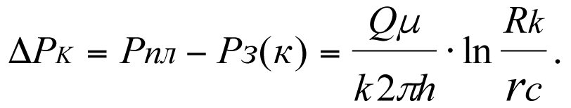 (3.4)
(3.4)
The additional loss of reservoir pressure, ∆Рs, that occurs in the skin layer with permeability factor ks during the filtration of the fluid to the bottom-hole region of a real-world is determined using the formula below (see Part 1, derivation of 1.13 and 1.35)
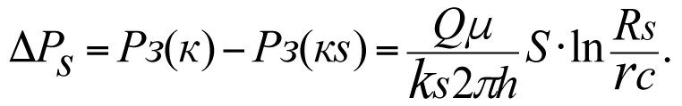 (3.5)
(3.5)
All notation items are explained in Fig. 3.1.

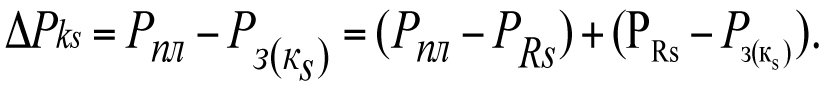
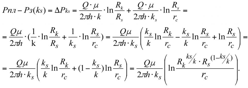
The total loss of reservoir pressure, ∆Рks, occurring in a multi-zone heterogenous reservoir (i. e. considering the skin layer) will equal
 (3.6)
(3.6)
or
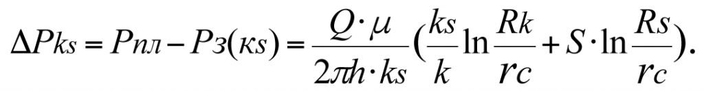 (3.7)
(3.7)
In Fig. 3.1, Curve 2 corresponds to equation (3.7). (3.7) gives us a formula for determining the volumetric influx rate (production flow rate) to the bottom-hole region of a hydrodynamically-imperfect (real-world) well
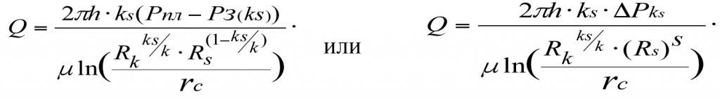 (3.8)
(3.8)
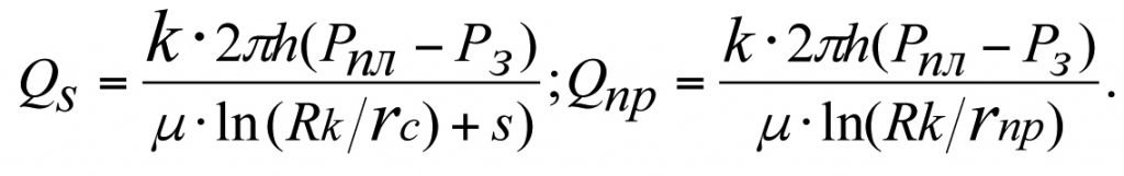
Variant 2. Determining the influx rate taking into account the pressure loss at the external boundary, Pпл-PRs, (Fig. 3.1, Curve 2); Q – const.
The pressure loss at the external boundary with permeability k will equal
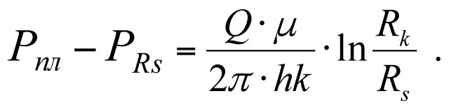 (3.9)
(3.9)
The pressure loss in the skin layer with permeability ks will equal
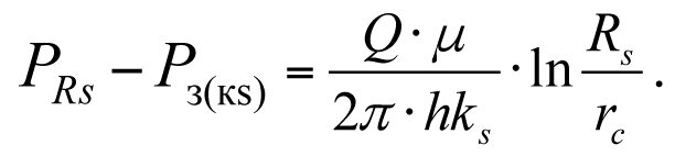 (3.10)
In this case, the total pressure loss in the near-wellbore region will equal
 (3.11)
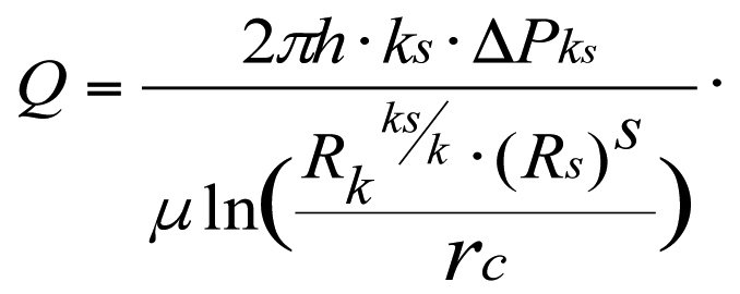
Plugging the values from (3.9) and (3.10) into (3.11), we obtain the pressure loss that occurs during fluid filtration in a multi-zone reservoir with heterogenous permeability distribution
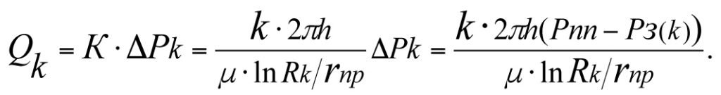
 (3.12)
 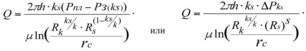 (3.13)
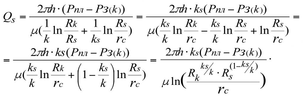
(3.12) gives us a formula for determining the influx rate to the bottom-hole region of a real-world well with heterogenous permeability distribution across the reservoir zones.
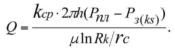
Variant 3. Determining the influx rate in a multi-zone heterogenous reservoir using its average permeability factor, kср, (Fig. 3.1). Q – const.
The production flow rate of an ideal well
 (3.14)
Let us express the flow rate of a real-world well using the average value of the permeability factor, kср. In this case, the reservoir is homogeneous and having permeability factor kср.
 (3.15)
Proceeding from the equality of the flow rates of the ideal and real-world wells and equating the right-hand sides of (3.14) and (3.15), we can write
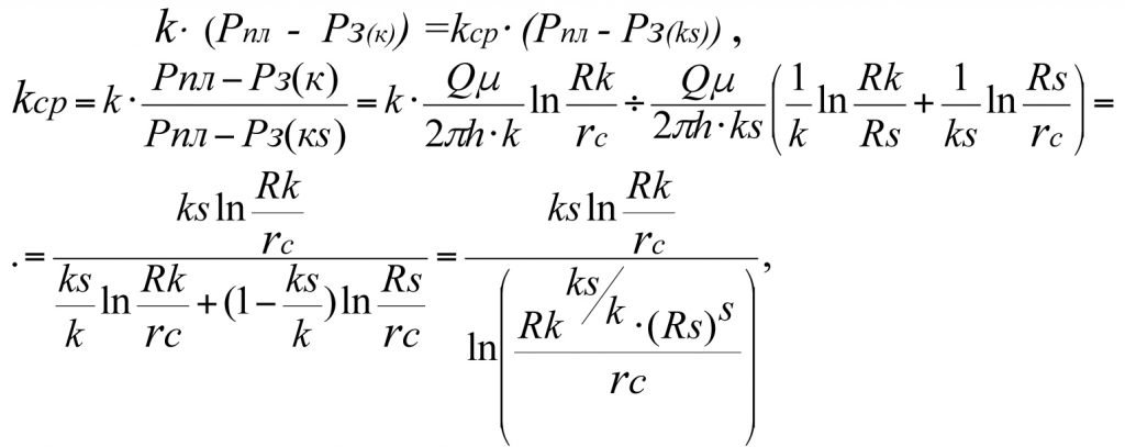
from which it follows that
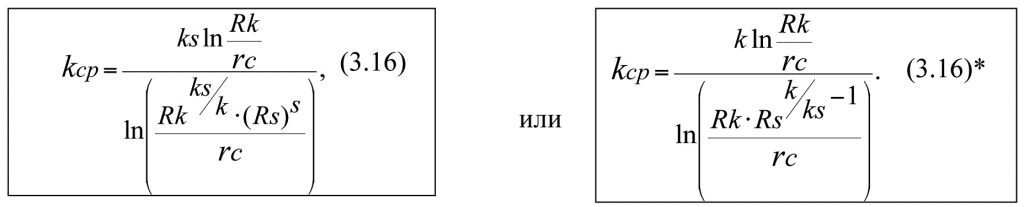
Formulas (3.16) and (3.16) * used for the determination of kср are equivalent.
Plugging the value from (3.16) into (3.15), we get the production flow rate of a real-world well with heterogenous permeability distribution across the reservoir zones
 (3.17)
Variant 4. Determining the production flow rate of a well with heterogenous permeability distribution across the reservoir zones given the equality in the bottom-hole pressure values, Рз(кs) = Pз(к)= Рз; Рпл – Рз(кs) = Рпл – Рз(к)=
=Рпл – Рз=ΔРk-const.
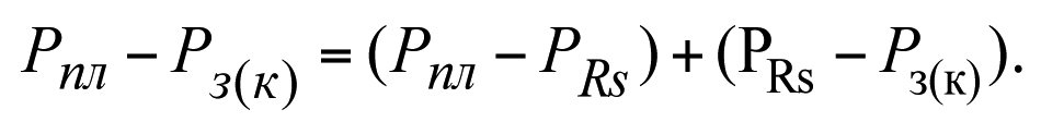
In the interval Рпл – РRs, the permeability factor is equal to k, and in the interval PRs –Pзк, it is equal to ks (see Fig. 3.1)
The total pressure loss in the interval Рпл – Рз(к)) will equal
 (3.18)
From (3.18) we get
 (3.19)
Formulas (3.8), (3.13), and (3.17) for determining the influx rate to the bottom-hole region of a well with heterogenous permeability distribution across the reservoir zones are identical, and (3.19) is equivalent.
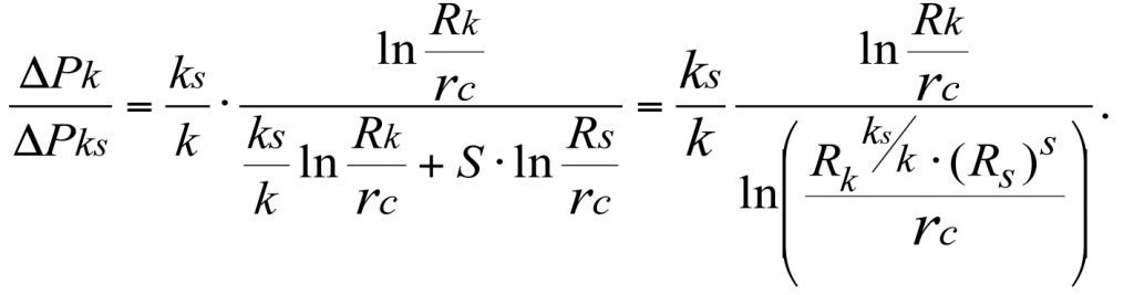
3.2. The drop in the rate of influx to the bottom-hole region of a real-world well occurring when the bottom-hole pressure decreases from Рз(k) to Рз(ks) (in a multi-zone reservoir with heterogenous permeability distribution)
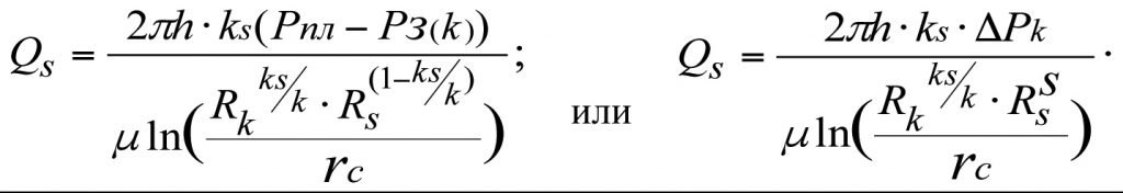
The influx rate at bottom-hole pressure Рз(ks) will equal (see 3.13)
 (3.20)
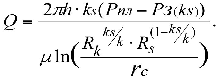
The influx rate at bottom-hole pressure Рз(k) will equal (see 3.19)
 (3.21)
In this case, the drop in influx rate will equal
ΔQ = Q – Qs,
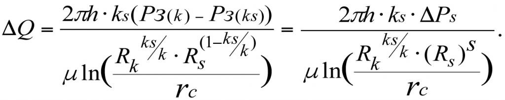
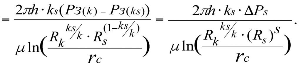 (3.22)
Formula (3.22) shows that a drop in pressure by ΔPs in the skin layer causes the influx rate (production flow rate) to decrease proportionally by ΔQ.
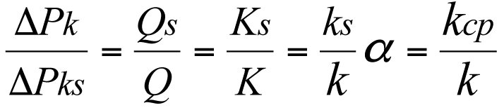
3.3. The relationship between the primary hydrodynamic parameters of the well and the reservoir permeability factor
3.3.1. The relationship between the productivity factor, Ks, of a real-world well and the permeability factor, ks, of a multi-zone heterogenous reservoir, Q-const.
The production flow rate of a real-world well in a multi-zone heterogeneous reservoir (3.8)
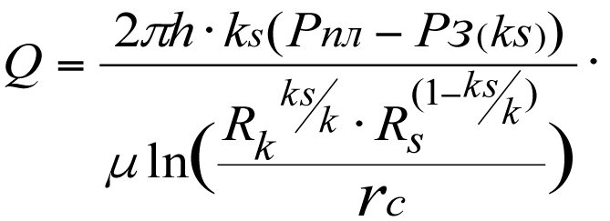 (3.23)
The production flow rate of an ideal well
 (3.24)
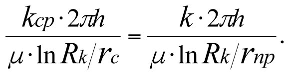
With Q-const, equating the right-hand sides of (3.23) and (3.24), we can write
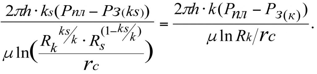
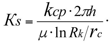
In this case, the productivity factor, Ks, of a real-world well will equal
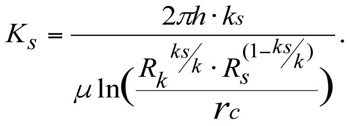 (3.25)
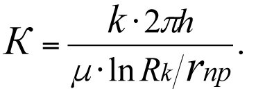
The productivity factor, K, of an ideal well
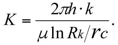 (3.26)
Dividing (3.25) by (3.26), we get
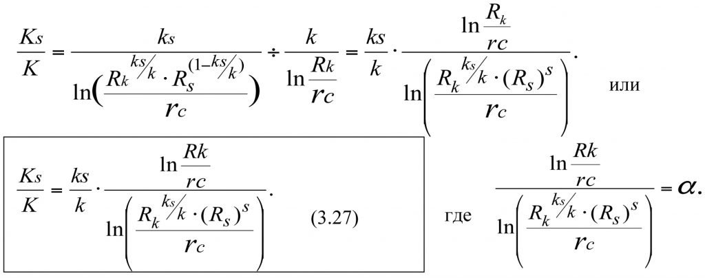 (3.27)
Let us introduce a new notation item, α, where α is the reservoir heterogeneity factor, i. e. a proportionality coefficient accounting for how non-homogeneously permeability is distributed within the reservoir.
In view of (3.16), we can write
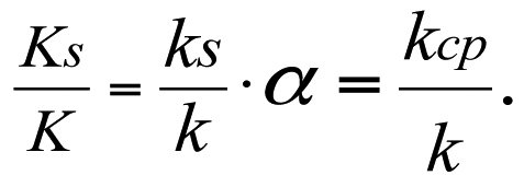 (3.28)
One important conclusion that follows from (3.28) is that the productivity factor of a real-world well, Ks, is directly proportional to the average permeability factor, kср, of a multi-zone heterogenous reservoir and that their relative values are equal to each other, whereas the skin zone permeability factor, ks, is directly dependent on the reservoir heterogeneity factor, α.
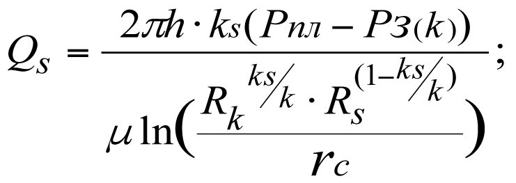
3.3.2. The relationship between the production flow rate of a real-world well, Qs, and the permeability factor, ks. Рз-const; (Рз(k)=Pз(ks)).
The production flow rate of a real-world well
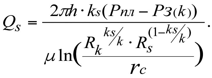
The production flow rate of an ideal well
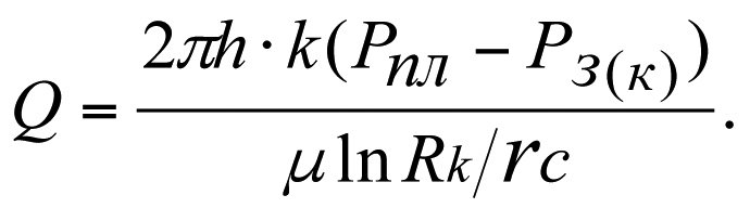
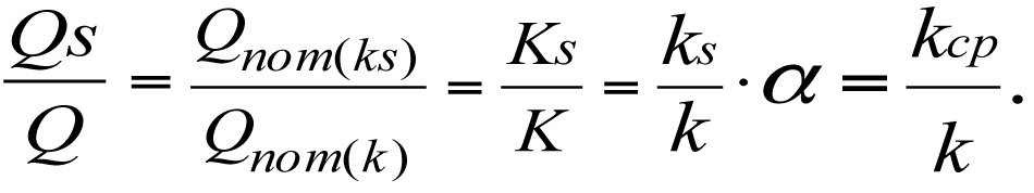
Dividing Qs by Q, we get
 or,
or,
in view of (3.16), we can write
 (3.29)
Formula (3.29) shows that the production flow rate of a real-world well, Qs, is directly proportional to the values of the factors ks, Ks, and kср, and their relative values are equal to each other.
3.3.3. The relationship between the permeability factor of a multi-zone heterogenous reservoir and the drop in reservoir pressure, ΔΡks, occurring during the filtration of the fluid, Q-const.
The loss of reservoir pressure, ΔΡk, that occurs during the filtration of the fluid to the bottom-hole region of an ideal well at reservoir permeability factor k is determined using the Dupuy formula
The total loss of reservoir pressure, ΔΡks, taking into account the skin layer, will equal
Dividing ΔΡk by ΔΡks, we get
In view of (3.16) and (3.29), we have
 (3.30)
Formula (3.30) shows that the total reservoir pressure loss, ΔΡks, occurring in a multi-zone heterogenous reservoir is inversely proportional to the values of Qs, Ks, ks, and kср, and their relative values are equal to each other.
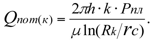
3.3.4. The relationship between the potential production flow rate, Qпот, of a heterogenous reservoir and its permeability factor.
The potential production flow rate of a real-world well given the multi-zone heterogeneity of the reservoir will equal
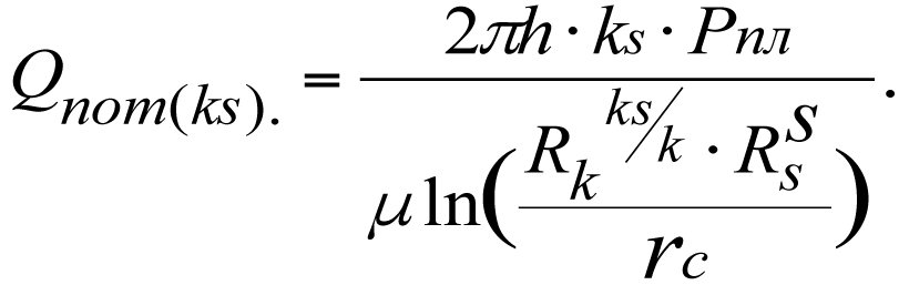
The potential production flow rate of an ideal well
Dividing Qпот(ks) by Qпот(k), we get
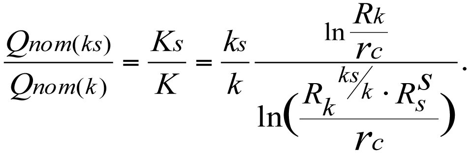
In view of (3.16) and (3.30), we can write
 (3.31)
The potential production flow rate, Qпот(ks) of a multi-zone heterogenous reservoir is directly dependent on its permeability, kср, and the relative values of Q, Qпот, K, ks, and kср are equal to each other.
3.4. Errors and misconceptions occurring in the theory of the effective (equivalent) wellbore radius, rпр
The commonest opinions and the things that everybody takes for granted deserve most often to be investigated.
Georg K. Lichtenberg. 1742–1799.
By definition, the equivalent wellbore radius, rпр ., is the borehole radius of an imaginary, fictitious, hydrodynamically-perfect well whose production flow rate is equal to the flow rate of a given hydrodynamically-imperfect well. Such a definition has been adopted in all scientific and educational publications, including non-Russian ones, relating to oil reservoir hydrodynamics. As we can infer from the definition,
Since the flow rates of the two wells are deemed to be equal (all other things being equal), we have
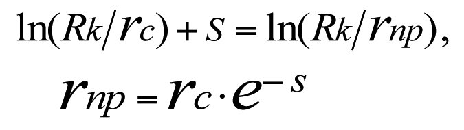 from which it follows that
(х *)
The untenability of this equivalent radius definition and of its formula (x*) follows from the fact that, theoretically, there are innumerable hydrodynamically-perfect fictitious wells with innumerable equivalent radius values whose production flow rates are, however, equal to each other and conformable to the flow rate of a given hydrodynamically-imperfect real-world well. This is well illustrated in Fig. 3.2. and in formula (3.32). For purposes of defining the equivalent radius and determining its value, the condition of equality of production flow rates between a hydrodynamically-imperfect real-world well and some fictitious, hydrodynamically-perfect well associated with it is, thus, an absolutely untenable and erroneous condition.
By applying different combinations of the productivity factor, Кi , and the bottom-hole pressure, Pзi, (i. e. drawdown, ΔРi), we can come up with innumerable fictitious wells with different equivalent radius values whose rates of influx to the bottom-hole region will, however, be equal to each other and conformable to the actual influx rate of a real-world well, see Fig. 3.2. and formula (3.32).

The infinite number of bottom-hole pressure values, Рз(i), corresponds to an infinite number of values of the productivity factor, К(i) and, hence, an infinite number of fictitious wells having different equivalent radii, rпр(i) but equal production flow rates.
 (3.32)
3.4.1. Defining the effective (equivalent) wellbore radius, rпр, and deriving its formula
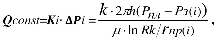
One value of the productivity factor, Kconst. corresponds to an infinite number of combinations of influx rate values, Qi, and reservoir drawdown values, ΔРi, i. e.
Kconst = Qi/ΔPi, from which it follows that
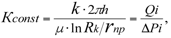 (3.33)
where Qi are different influx rate values corresponding to different reservoir drawdown values, ΔPi = Рпл – Рз(i), in the case of fictitious wells, rпр being the equivalent borehole radius of the fictitious well.
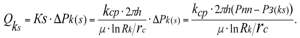
The let us express the production flow rate of a real-world well in a multi-zone heterogenous reservoir in terms of the average value of the permeability factor, kср (see 3.16). In this case, the reservoir is considered to be homogeneous and having permeability factor kср.
 (3.34)
The notation is as shown in Fig. 3.2. and 3.3.

The production flow rate of a perfect, fictitious well (Curve 1 in Fig. 3.3)
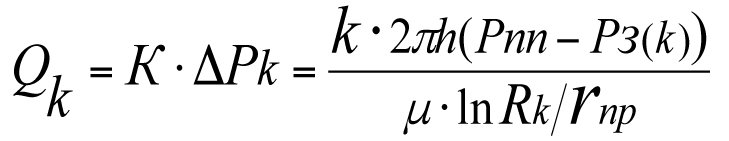 (3.35)
When the productivity factors of the real-world well Кs and the fictitious well (К) are equal to each other (Кs=К), the indicator lines Q=f(ΔP) of these wells will coincide. At the same time, the reservoir drawdown can take many different values, (ΔРк>ΔРк(s)), (ΔРк<ΔРк(s)), (ΔРк=ΔРк(s)), corresponding to different influx rate values, Qi. In the special case where the reservoir drawdown values for the real-world well and the fictitious well are equal to each other ΔРк=ΔРк(s), see Fig. 3.2 and 3.3), the production flow rates of these wells will also be equal.
Formula (3.33) makes it clear that the values of Qi and ΔPi can be combined in an innumerable of ways to produce the same value of the productivity factor, while the effective (equivalent) radius, rпр, is associated only with the productivity factor, К, of the fictitious well.
Based on an analysis of formulas (3.33), (3.34), and (3.35) as well as of Fig. 3.2 and 3.3, we can conclude that, all other things being equal, a unique value of the productivity factor corresponds to a unique value of the effective (equivalent) borehole radius of a fictitious well.
Hence, the following definition for the effective (equivalent) wellbore radius is proposed:
The effective (equivalent) wellbore radius is the borehole radius of a hydrodynamically-perfect fictitious well whose productivity factor is equal to the productivity factor of a hydrodynamically-imperfect real-world well.
A necessary and sufficient condition for determining the effective (equivalent) borehole radius, rпр, of a hydrodynamically-perfect well associated with some real-world well is, thus, that the values of the productivity factors of the latter (Кs) and the former (К) wells be equal to each other.
The production flow rate of a hydrodynamically-imperfect (real-world) well from (3.34)
 (3.36)
The productivity factor of a real-world well
 (3.37)
The production flow rate of a hydrodynamically-perfect fictitious well from (3.35)
 (3.38)
The productivity factor of a fictitious well
 (3.39)
The productivity factors of the real-world and fictitious wells being equal, we have
 (3.40)
(3.40) gives us a formula for determining the effective (equivalent) wellbore radius, rпр
 (3.41)
The average value of the permeability factor, kср, is determined using formula (3.16).
(3.41) makes it clear that the value of the equivalent borehole radius, rпр, of a fictitious well depends on the ratio between the radius of the borehole of the real-world-well and the radius of the external reservoir boundary appearing in the exponent part of an exponential function. When the permeability factors of the external reservoir boundary of a real and a fictitious well are equal (i.e. in the absence of a skin zone, k=kср) their radii will also be equal.
Epilogue From the Author
The multifaceted science of subsurface hydrodynamics, which embraces the laws of Newton’s mechanics and quantum mechanics [9], cannot be logically completed, it can only be cut off for a while.
The problems that have been considered in my works are related to the fundamental tenets of subsurface hydrodynamics. The historical errors and misconceptions that are present in the formulas for determining the pressure loss ΔРs during the filtration of wellbore fluid in the near-wellbore space, the values of the skin factor, S, productivity factor, К, bottom-hole pressure, Рз, dynamic level of wellbore fluid, hд, current influx rate, Qж, potential production flow rate, Qпот, and effective (equivalent) wellbore radius, rпр, all stem from one and the same chain of errors. The negative consequences of these errors and delusions have been reflected in the theory and practice of the fundamentals of hydrodynamic well testing (GDIS), geophysical well logging (GIS), and mud logging (TIS), but something we can really describe as a disastrous effect is the fact that, since the second half of the last century, these formulas have been included in all textbooks, teaching aids, and study guides of universities, colleges, and postgraduate training courses specializing in the subject-matter without any derivations or proofs whatsoever.
What is extremely surprising is that some of the leading ideologists of wellbore hydrodynamics research such as A. I. Ipatov, M. I. Kremenetsky, and D. N. Gulyayev [7] consider the formulas in A. F. van Everdingen & N. Hurst, 1949 (1*) and M. F. Hawkins, 1956 (2 *), which were composed contrary to the laws of subsurface hydrodynamics and contain gross mathematical errors, to be the classics and to represent fundamental tenets of well testing.
Formulas (1 *) and (2 *) used for determining ΔРs and S as well as formulas (3.2), (3.2*), (3.3), and (3.3 *) used for calculating Qж and the effective (equivalent) wellbore radius, rпр (x *), are not suitable for calculating the said fundamental hydrodynamic parameters of a real-world well characterized by heterogeneous permeability distribution across the reservoir zones and should be removed from textbooks and teaching aids in subsurface hydrodynamics.
The fundamental dependences between the hydrodynamic parameters of the “Reservoir – Well – Pumping Equipment” system should be used to quantify and fully analyze the state of the reservoir, as well as for purposes of hydrodynamic well testing (GDIS), geophysical well logging (GIS), mud logging (TIS), and comprehensive technological and hydrodynamic feasibility assessments for software development projects to support innovative process design solutions for oil and gas field development.
As a branch or science, subsurface hydrodynamics is far from perfect and, by the end of the 1950s, it had almost completely exhausted its potential. Since that time, no fundamental theories have been created, and the conceptual developments that took shape along the main avenues of application have indeed gone the wrong way. Modern subsurface hydrodynamics is ailing from the inside out. The main causes of that ailment, as well as its tenacity and persistence, are a profound stagnation in scientific ideas combined with a dogmatic approach to formulating and solving fundamental scientific problems aggravated by the conservatism of scientific thought. Whatever research work was conducted in the field of subsurface hydrodynamics since that time up until the present day can be reduced to the development of semi-empirical theories whose sole purpose was to tweak the mathematical apparatus to reality and which, as all erroneous concepts, had but preparatory value if any.
Some yet-unanswered questions of hydrodynamics
A producing reservoir is exposed to a multitude of changing geophysical fields (multi-fields): geomechanical, hydrodynamic, geomagnetic, electrodynamic, geothermodynamic, gravitational, undulatory, optical, as well as their derivatives. The values of the parameters of these geophysical fields are fully interlinked with all the hydrodynamic parameters of the reservoir and depend on the spatial heterogeneity and temporal variability of the state of the entire system [9].
The following tenets of subsurface hydrodynamics require answers:
– determination of interrelation between all of the specified parameters and their values;
– filtration of formation fluid under the action of multi-fields;
– effect of those fields on its rheological properties;
– interrelation of the formation gravity and the magnetic field of a formation;
– increment of formation entropy in the process of field development.
All of these questions asked by the nature itself can only be answered within the framework of the laws of quantum mechanics.
Besides, certain experiments on turbulent fluid flows conducted by I. Nikuradze have shown that there are inconsistencies between the experimental data gathered and theoretical predictions made about the viscous sublayer of the boundary zone. To eliminate the inconsistencies, the paper introduced several empirical constants such as the “kinetic energy defect,” “total head defect,” and “velocity defect.” These “defects” can be remedied within the framework of quantum mechanics.
It should be noted that all classical conservation laws have quantum analogues, and conversely, there are quantum conservation laws that have no analogues in classical physics.
All scientific and technological advances are made possible by fundamental ideas and discoveries that form their vanguard. Any errors and delusions that slip into the fundamental and pivotal branches of science always lead to dead ends and translate into enormous costs incurred throughout the implementation process, from the initial idea to the final production runs.
The author will appreciate reasonable and well-substantiated comments and suggestions affecting the structure and content of the final formulas and clarifying the definitions.
Brief information about the author:
Robert Mufazalov
– 275 academic papers, of which:
– 117 inventions;
– 13 monographs (scientific books);
– 4 university textbooks (endorsed by the Ministry of Higher Education);
– Honored Inventor of the Republic of Bashkortostan;
– Inventor of the USSR;
– Excellence Award from the Ministry of Oil Industry of the USSR;
– Mentioned in the encyclopedia titled “Engineers of the Urals»;
– Corresponding Member of the Academy of Natural Sciences;
– Participant of more than 30 international conferences, congresses, and international exhibitions on the latest and research-intensive technology.
Academic interests: quantum geomechanics, subsurface hydrodynamics, hydraulics, nonlinear hydroacoustics, drilling equipment and technology, oil production hydromechanics, petrochemistry, medicine (8 patents for inventions), development and creation of high technology for the petrochemical complex.
Bibliography
1. A. F. van Everdingen and W. Hurst. The Application of the Laplace Transformation to Flow Problems in Reservoirs. – Trans. AIME, Vol. 186, 1949. – pp. 305–24.
2. M. F. Hawkins, Jr. A note on the skin effect. – Trans. AIME, Vol. 207, 1956. – pp. 356–57.
3. Справочное руководство по проектированию разработки и эксплуатации нефтяных месторождений // Под общ. ред. Ш. К. Гиматудинова. – М.: Недра, 1983. – 455с. [Reference guide to the design of oilfield development and production projects // Under the general editorship of Sh. K. Gimatudinov. – Moscow: Nedra, 1983. – 455 pp.]
4. Ипатов А. И., Кременецкий М. И. Геофизический и гидродинамический контроль разработки месторождений углеводородов. – Изд. 2-е, испр. – М.: НИЦ «Регулярная и хаотическая динамика», 2010. – 780с. [A. I. Ipatov, M. I. Kremenetsky. Geophysical and hydrodynamic monitoring of the development of hydrocarbon fields. – 2nd revised edition. – Moscow: Regular and Chaotic Dynamics Research Center, 2010. – 780 pp.]
5. Закиров С. Н., Индрупский И. М., Закиров Э. С. и др. Новые принципы и технологии разработки месторождений нефти и газа. Часть 2. – М. – Ижевск: Институт компьютерных исследований, НИЦ «Регулярная и хаотичная динамика», 2009. – 484 с. [S. N. Zakirov, I. M. Indrupsky, E. S. Zakirov, et al. New principles and technologies for the development of oil and gas fields. Part 2. – Moscow – Izhevsk: Institute for Computer Research, Regular and Chaotic Dynamics Research Center, 2009. – 484 pp.]
6. Щуров В. И. Технология и техника добычи нефти. Учебник для вузов. – М.: Недра, 1983. – 510 с. [V. I. Shchurov. Oil production technology and equipment. Textbook for institutions of higher education. – Moscow: Nedra, 1983. – 510 pp.]
7. Ипатов А. И., Кременецкий М. И., Гуляев Д. Н. Современные технологии гидродинамических исследований скважин и их возрастающая роль в разработке месторождений углеводородов // Нефтяное хозяйство. – 2009. – № 5. – С. 52–57. [A. I. Ipatov, M. I. Kremenetsky, D. N. Gulyayev. Modern technologies for hydrodynamic well testing and their increasing role in the development of hydrocarbon fields // Neftyanoye Khozyaystvo. – 2009. – # 5.
– pp. 52–57.]
8. Муфазалов Р. Ш. Скин-фактор. Исторические ошибки и заблуждения, допущенные в теории гидродинамики нефтяного пласта. – Георесурсы.
№ 5. – 2013. – С. 34–48. [R. Sh. Mufazalov. Skin factor. Historical errors and misconceptions at work in the oil reservoir hydrodynamics theory. – Georesources. Issue # 5. – 2013. – pp. 34–48.]
9. R. Sh. Mufazalov. Fundamentals of Subsurface Hydrodynamics and a Quantum-Mechanical View of the Reservoir Model // «ROGTEC», Oil & Gas Magazine, Issue # 55. – рр. 44–59. (Tel: +34 952 880 952, editorial@rogtecmagazine.com, Spain).
10. R. Sh. Mufazalov. Tim’s Theorem: A New Paradigm for Underground Hydrodynamics. Part 1 // «ROGTEC», Oil & Gas Magazine, Issue # 57. – рр. 62–78. (Tel: +34 952 880 952, editorial@rogtecmagazine.com, Spain).
11. Муфазалов Р. Ш. Скин-фактор и его значение для оценки состояния околоскважинного пространства продуктивного пласта. – Уфа: Изд-во УГНТУ. – 2005. – 44 с. [R. Sh. Mufazalov. Skin factor and its significance for assessing the state of the near-wellbore region of a producing reservoir. – Ufa: UGNTU Publishing House. – 2005. – 44 pp.]